Multi-Layer Perceptron (MLP) with Keras

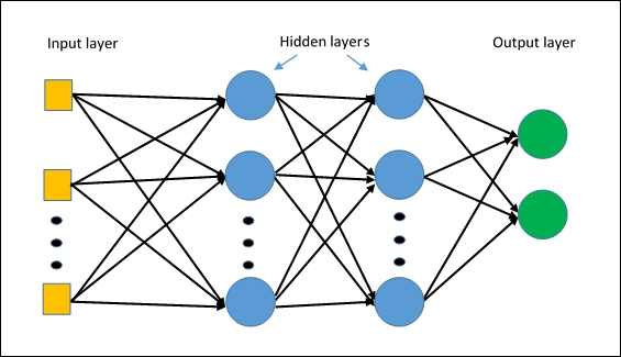
Multi-Layer Perceptron is famous nowadays as we have enough processing power to compute heavy operations. It consists of 3 layers: input, hidden and an output layer. In this post, we will implement the neural network with Keras. Keras is a python deep learning library.

In the dataset, we have ASCII representation, where each letter of the alphabet is represented by a matrix of 12x13 binary values. Here, we will train our model and check the analyze the learning curve.

So first we will import the required packages and load the data.

import numpy as np
from keras import models, layers, optimizers, utils
from random import randint
from keras.layers.core import Activation
from keras.layers import Dropout
from matplotlib import pyplot as plt

dataset = np.loadtxt('pattern1.txt', delimiter=" ")

In our data file, we have A to Z letter, so we will transform our data first and then split the train and test data. We’ll also prepare our target column as in form of ASCII values. In our case, we have limited data, so we will take some letters randomly from the training data and use it as test data. In a real-world application, we use unseen data for the validation and test data set.

def oneRowTransform(dataset):
    
    temp = []
    x_data = []
    startIndex = 0
    distance = 12
    endIndex = distance

    for i in range (int(len(dataset)/12)): 
    
        temp = dataset[startIndex: endIndex]
        startIndex = endIndex
        endIndex = startIndex + distance
        x_data.append(temp)
        temp = []
        
    x_temp = []
    for number in range(len(x_data)):
        flat_list = [item for sublist in x_data[number] for item in sublist]
        x_temp.append(flat_list)
        
    return x_temp

x_temp = oneRowTransform(dataset)

x_test, y_test  = [], []
y_data = utils.to_categorical(list(range(65,91))).tolist()

tempList_x = list(x_temp)
tempList_y = list(y_data)

# splitting train and test data. Further transformation operation 
for i in range(8):
    randomNumber = randint(0, len(x_temp)-1)
    x_test.append(x_temp[randomNumber])
    y_test.append(y_data[randomNumber])
    x_temp.pop(randomNumber)
    y_data.pop(randomNumber)
    
x_train = np.array(tempList_x).reshape(26,156)
x_test = np.array(x_test).reshape(8,156)

y_train = np.array(tempList_y)
y_test = np.array(y_test)

Now coming to building the model, we will have 3 layers: an input layer, an output layer and 1 hidden layer.

def MLPmodel(node, x_train, y_train, x_test, y_test, epochs, batch_size):
    
    model = None
    model = models.Sequential()
    
    model.add(layers.Dense(node, input_dim=156))
    model.add(Activation('relu'))
    model.add(Dropout(0.15))
    
    model.add(layers.Dense(node))
    model.add(Activation('relu'))
    model.add(Dropout(0.15))
    
    model.add(layers.Dense(91))
    model.add(Activation('softmax'))
    model.summary()
    model.compile(loss='categorical_crossentropy',
                  optimizer=optimizers.Adadelta(), metrics=['accuracy'])
    
    test = model.fit(x_train, y_train,
              batch_size=batch_size,
              epochs=epochs,
              verbose=0,
              validation_data=(x_test, y_test))
    score = model.evaluate(x_test, y_test, verbose=0)
    prediction = model.predict_classes(x_test, verbose=0)
    
    return test, score, prediction, model

We have used ‘relu’ and ‘softmax’ as an activation function for our layers. Dropout is for setting a fraction of input units to zero during the training time. It helps to prevent overfitting especially when we are dealing with letter recognition problem and if our network is large and complex then there are chances that one neuron unit might get trained to a certain level of input. To prevent this, we are turning off the unit randomly so train the other part of the network with noisy data. Lost function and optimization techniques can differ (gradient descent in case of linear regression).

We are validating our model against the training data, again it has to unseen data for the generalized model.  Then we’ll be evaluating the model against the test data.

Now, let’s just build the model and see the results.

test, score, prediction, model = MLPmodel(128, x_train, y_train,
                                   x_test, y_test, 25, 10)  

print('Test loss:', score[0])
print('Test accuracy:', score[1])

We’ll plot the accuracy graph of training and validation accuracy against the number of epochs to check whether our model is overfitting or not.

def lineGraph(firstValue, secondValue, firstMarker, secondMarker,
               lineOne, lineTwo, colorOne, colorTwo, title, 
               labelOne, labelTwo, x_label, y_label):
    
    plt.plot(firstValue, marker=firstMarker, linestyle=lineOne, 
                 color=colorOne, label=labelOne)
    plt.plot(secondValue, marker=secondMarker, linestyle=lineTwo, 
                 color=colorTwo, label=labelTwo)
    plt.xlabel(x_label)
    plt.ylabel(y_label)
    plt.title(title)
    plt.legend()
    plt.show()

lineGraph(test.history['acc'], test.history['val_acc'], 'x', 'o', 
          '-','--', 'b','r', 'Training Data vs Validation Data Accuracy',
         'Training Set Accuracy','Validation Set Accuracy','No of Epoch','Accuracy')

Based on the graph, we can say that validation accuracy is higher than the training accuracy which means its not the case of overfitting.

Find the complete Jupyter Notebook and dataset here.

Subscribe my blog for the further technical guide. Cheers!